MatPower Wrapper - Example and Documents
This work presents wrapper-based interfaces to integrate industry modeling tools targeted to specific functions within co-simulation (co-sim). These interfaces leverage MATPOWER-MOST, developed to minimize the barrier for simulating wholesale market operations and thereby facilitate comprehensive evaluation of candidate DER coordination schemes for providing grid services. The wrapper presented herein contains several programming language functions (PLFs) that encapsulate the complex formatting and coordination requirements between market processes and organizes the co-sim-based information exchange with other platforms working in tandem. The wrapper aims to provide open-source easy-to-use configurable interfaces for researchers and students to reduce the modeling complexity inherent to market operations while maintaining detailed emulation of the system. The wrapper-based interfaces are implemented on an 8-bus test system representing ERCOT to demonstrate its capabilities to model wholesale market operations and evaluate the impact of flexible resources such as DERs. This tool utilizes the existing open-source tool, Matpower, which is compatible with both MatLab and Octave. Hereafter, references to MatLab can be considered to also apply to Octave unless explicitly stated.
It is assumed that a user for this tool has already installed:
Either GUROBI or Mosek (optional, but running unit commitment is not advised without these; GUROBI reccomended)
Wrapper Architecture
The wrapper itself contains functions to facilitate day-ahead (DA) and real-time (RT) market emulations as well as power flow emulations and functions to help interact with the co-simulation platform HELICS. These components are outlined in Figure Fig. 59.
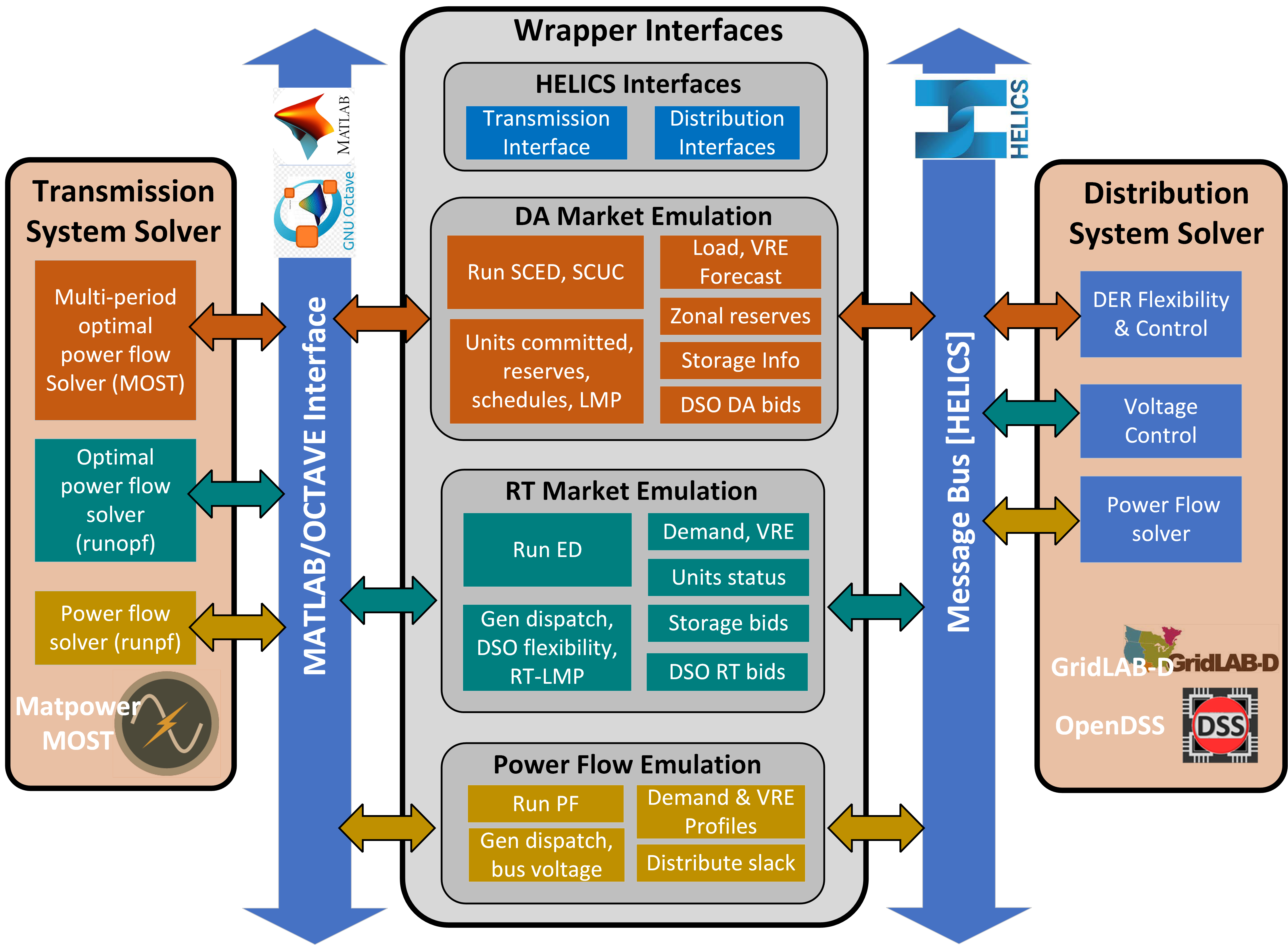
Fig. 59 High-level wrapper architecture diagram
Initial Setup
The wrapper uses a few setup files to define the settings for the simulation being run.
The “wrapper_startup.m” file is where the user can define the needed paths for Matpower, HELICS, and whichever solver they wish to use (Mosek, GUROBI, etc.).
The “helics_config.json” file is automatically generated by the “prepare_helics_config” function based on which components are defined to used in a given. “Publications” define the data being sent from the MatLab side such as clearing price for a market or voltage setpoints for a powerflow. “Subscriptions” defines the data being sent to the market simulator from an external source such as energy bids or updated loads due to a decision made about a battery control.
The “wrapper_config.json” file is the primary configuration file for the wrapper and contains the majority of the settings for the wrapper. This is where the user defines elements such as the location of the data used to set up the model used in the simulation as well as any load or generation profiles to be used. The basic settings are also contained in this file, including the timeframe to be simulated, which emulations should be included (powerflow, RT Market, and/or DA market) and how often they should run. This file contains the settings for utilizing HELICS for co-simulation or to include a locally-defined storage component.
The “storage_config.json” file allows for user-defined storage elements to be added to the simulation; defining energy capacity, power capacity, round-trip efficiency, and location (via bus number).
Day-Ahead Market
- get_DAM_bids_from_wrapper(obj, time, flexiblity_profile, price_range, blocks): Used when not relying on co-simulation for DA generator bids. Bids are taken from local files.
Inputs
obj: The MatPower Wrapper object
time: Currently unused in this function; The load profile for the upcoming day is taken from the Wrapper object
flexiblity_profile: An array of 24 values representing the fraction of the load at the given cosimulation bus that is part of the flexible load. The fractions are represented as decimals, so a profile with 20% flexibility for the entire day would look like [0.2, 0.2, 0.2, …]. A profile with 10% flexibility from midnight to 1am, 20% flexibility from 1am to 2 am, and 0% flexibility for the rest of the day would look like [0.1, 0.2, 0.0, 0.0, …]. (Both arrays have a total of 24 values representing each hour of the day)
price_range: An array with 2 numerical values representing the minimum and maximum prices to use for flexible load bids.
blocks(positive integer): The number of bidding blocks to be created for the flexible load bids.
Example: for a given hour of the day with a flexibility profile value of 0.2 where price_range=[20,50] and blocks=4
If the price<20, none of the flexible load will be shed
If 20<price<30, 5% of the load will be shed
if 30<price<40, 10% of the load will be shed
if 40<price<50, 15% of the load will be shed
if price>50, 20% of the load will be shed
Where price is in $/MWHr
Output
The MatPower Wrapper object will have updated values for obj.DAM_bids for the entry representing the cosimulation bus defined in wrapper_config.json
- get_DA_forecast(obj, input_fieldname, current_time, interval): Forecasted load values for the next day are taken from local files.
Inputs
obj: The MatPower Wrapper object
input_fieldname: a string representing which profile is being updated (accepted inputs: ‘load_profile’, ‘wind_profile’, or ‘solar_profile’).
current_time: the time in seconds from the start of the simulation.
interval: the separation between DA markets in seconds. (must match what was defined in wrapper_config.json, suggest just passing in Wrapper.config_data.day_ahead_market.interval)
Output
Updates obj.forecast.(input_fieldname) for the coming day with the data stored in obj.profiles.(input_fieldname)
Real-Time Market
- get_RTM_bids_from_wrapper(obj, time, flexiblity_profile, price_range, blocks): Used when not relying on co-simulation for RT generator bids. Bids are taken from local files.
Inputs
obj: The MatPower Wrapper object
time: Currently unused in this function; The load profile for the upcoming time interval is taken from the Wrapper object
flexiblity_profile: An array of 24 values representing the fraction of the load at the given cosimulation bus that is part of the flexible load. The fractions are represented as decimals, so a profile with 20% flexibility for the entire day would look like [0.2, 0.2, 0.2, …]. A profile with 10% flexibility from midnight to 1am, 20% flexibility from 1am to 2 am, and 0% flexibility for the rest of the day would look like [0.1, 0.2, 0.0, 0.0, …]. (Both arrays have a total of 24 values representing each hour of the day)
price_range: An array with 2 numerical values representing the minimum and maximum prices to use for flexible load bids.
blocks(positive integer): The number of bidding blocks to be created for the flexible load bids.
Example: for a given hour of the day with a flexibility profile value of 0.2 where price_range=[20,50] and blocks=4
If the price<20, none of the flexible load will be shed
If 20<price<30, 5% of the load will be shed
if 30<price<40, 10% of the load will be shed
if 40<price<50, 15% of the load will be shed
if price>50, 20% of the load will be shed
Where price is in $/MWHr
Output
The MatPower Wrapper object will have updated values for obj.RTM_bids for the entry representing the cosimulation bus defined in wrapper_config.json
- run_RT_market(obj, time): Runs a RT market with the current wrapper configuration.
Inputs
obj: The MatPower Wrapper object
time: The starting time for the Real-Time market interval to be run in seconds from the start of the simulation(as defined in wrapper_config.json).
Example: time=900 would run a RT market starting at 12:15 am (900 seconds = 15 minutes) on the first day of the simulation
Output
Populates obj.results.RTM with the results of the market simulation for the defined time period. Results include output for each generator as well as demand and marginal prices at each bus.
Power Flow
- run_power_flow(obj, time): Runs a power flow with the current wrapper configuration.
Inputs
obj: The MatPower Wrapper object
time: The starting time for the power flow interval to be run in seconds from the start of the simulation(as defined in wrapper_config.json).
Example: time=1200 would run a power flow starting at 12:20 am (1200 seconds = 20 minutes) on the first day of the simulation.
Output
Updates obj.mpc.bus(:,8:9) which represents the voltage magnitude and angle for each bus and obj.mpc.gen(:,2:3) which represents real and reactive power output for each generator. Also adds to obj.results.PF.VM which records the time and voltage magnitudes for each bus.
HELICS Interfaces
- prepare_helics_config(obj, config_file_name, SubSim): Creates the “helics_config.json” file based on your settings in other configuration files.
Inputs
obj: The MatPower Wrapper object
config_file_name: a string to be used in naming the configuration file (referred to as ‘helics_config.json’ here and in the example)
SubSim: a string to be used at the beginning of the Helics subscription keys. Used for naming the keys only; see Helics documentation for more information.
Output
Creates the Helics configuration file with the name specified by config_file_name using the settings defined in “Wrapper_config.json”
No explicit output within MatLab
- start_helics_federate(obj, config_file_name): Beings the federate, allowing communication through HELICS to begin.
Inputs
obj: The MatPower Wrapper object
config_file_name: a string matching the imput used in prepare_helics_config
Output
Updates obj.helics_data.(‘fed’) with the federate object
Updates obj.helics_data.(‘pub_keys’) with a list of Helics publication keys
Updates obj.helics_data.(‘sub_keys’) with a list of Helics subscription keys
Helics federate starts (See Helics documentation for further context)
- get_storage_from_helics(obj): Reads in storage specs from the co-simulation rather than using the values defined in storage_config.json.
Inputs
obj: The MatPower Wrapper object
Output
Updates obj.storage_specs with the specifications sent from the co-simulation. The co-simulation should send a string in the format of a .json file. “storage_config.json” gives an example for the specs of two batteries located at bus 2, with 500MWHr capacities, 250MW maximum charging/discharging, and 96% and 93% round-trip efficiencies repsectively.
- get_loads_from_helics(obj): Receives updated load information for the current time for the defined co-simulation bus(es) as defined in wrapper_config.json.
Inputs
obj: The MatPower Wrapper object
Output
Updates obj.mpc.bus(,3:4) with the real and imaginary components of the load at each cosimulation bus based on the complex values passed through Helics.
- send_voltages_to_helics(obj): Sends cleared voltages for the defined co-simulation bus(es) from the last power flow.
Inputs
obj: The MatPower Wrapper object
Output
No explicit output within MatLab. Sends the cleared volatges for the cosimulation buses from last power flow through Helics.
- get_RTM_bids_from_helics(obj): Receives generator bids for the real-time market sent from HELICS.
Inputs
obj: The MatPower Wrapper object
Output
Updates obj.RTM_bids for each cosimulation bus based on the string recieved from the cosimulation through HELICS.
- get_DAM_bids_from_helics(obj): Receives generator bids for the day-ahead market sent from HELICS.
Inputs
obj: The MatPower Wrapper object
Output
Updates obj.DAM_bids for each cosimulation bus based on the string recieved from the cosimulation through HELICS.
- send_DA_allocations_to_helics(obj): Sends the generator allocations from the last day-ahead market to HELICS.
Inputs
obj: The MatPower Wrapper object
Output
No explicit output within MatLab. Sends the content of obj.RTM_allocations as a string in .json format for each cosimulation bus through HELICS.
- send_RTM_allocations_to_helics(obj): Sends the generator allocations from the last real-time market to HELICS.
Inputs
obj: The MatPower Wrapper object
Output
No explicit output within MatLab. Sends the content of obj.DAM_allocations as a string in .json format for each cosimulation bus through HELICS.