Design Reference

Messages between Simulators and Agents

TESP simulators exchange the sets of messages shown in Fig. 59 and Fig. 60.

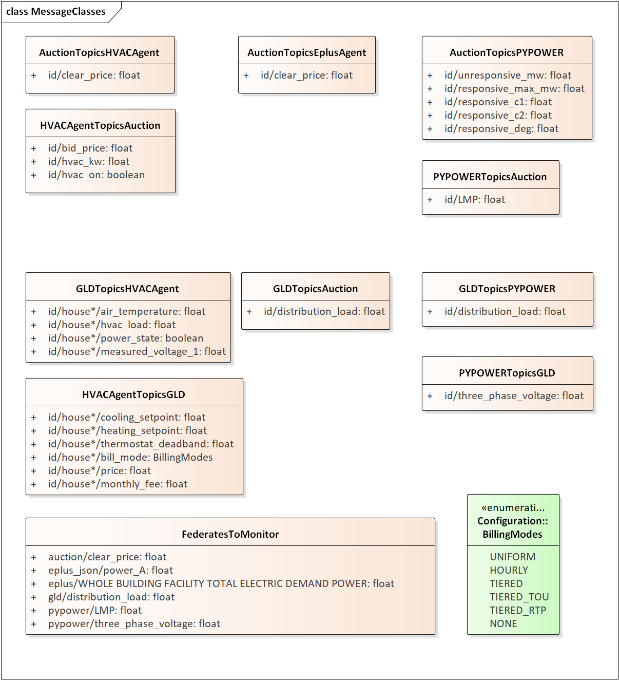
Fig. 59 Message Schemas for GridLAB-D, PYPOWER and residential agents

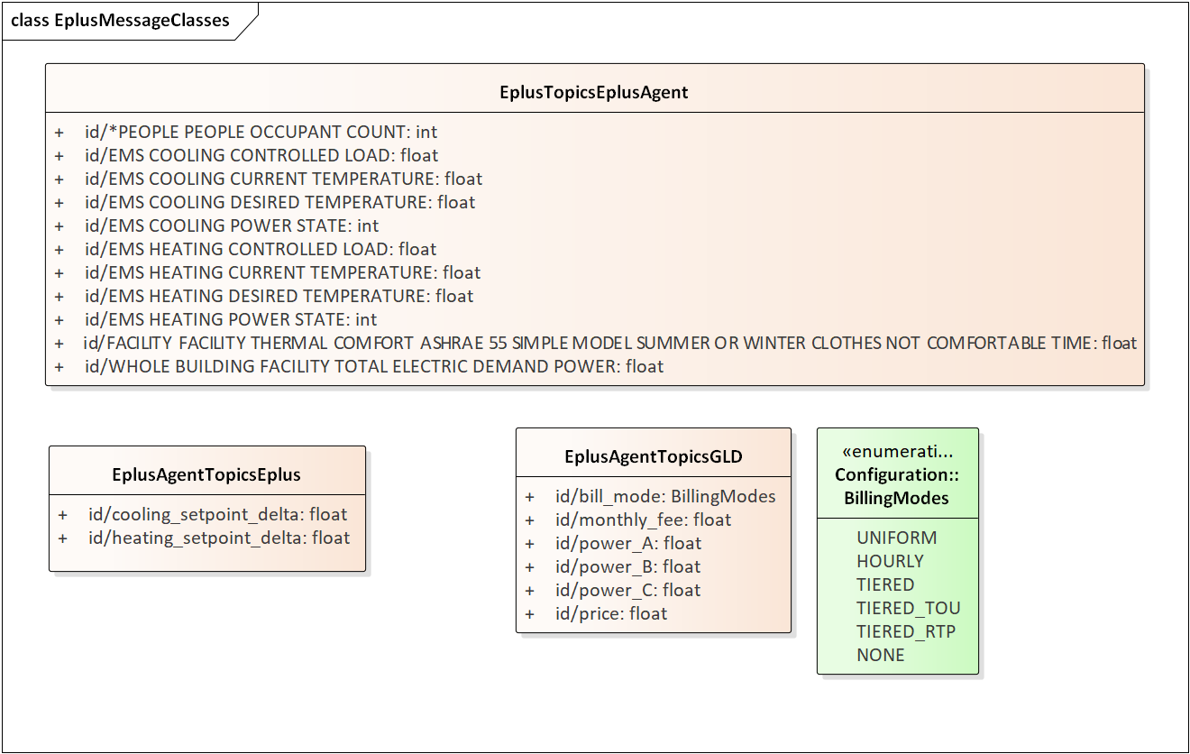
Fig. 60 Message Schemas for EnergyPlus and large-building agents

These messages route through HELICS in a format like “topic/keyword=value”. In Fig. 61, the “id” would refer to a specific feeder, house, market, or building, and it would be the message topic. Once published via HELICS, any other HELICS simulator can access the value by subscription. For example, PYPOWER publishes two values, the locational marginal price (LMP) at a substation bus and the positive sequence three-phase voltage at the bus. GridLAB-D subscribes to the voltage, using it to update the power flow solution. The double-auction for that substation subscribes to the LMP, using it to represent a seller in the next market clearing interval. In turn, GridLAB-D publishes a distribution load value at the substation following each significantly different power flow solution; PYPOWER subscribes to that value for its next optimal power flow solution.

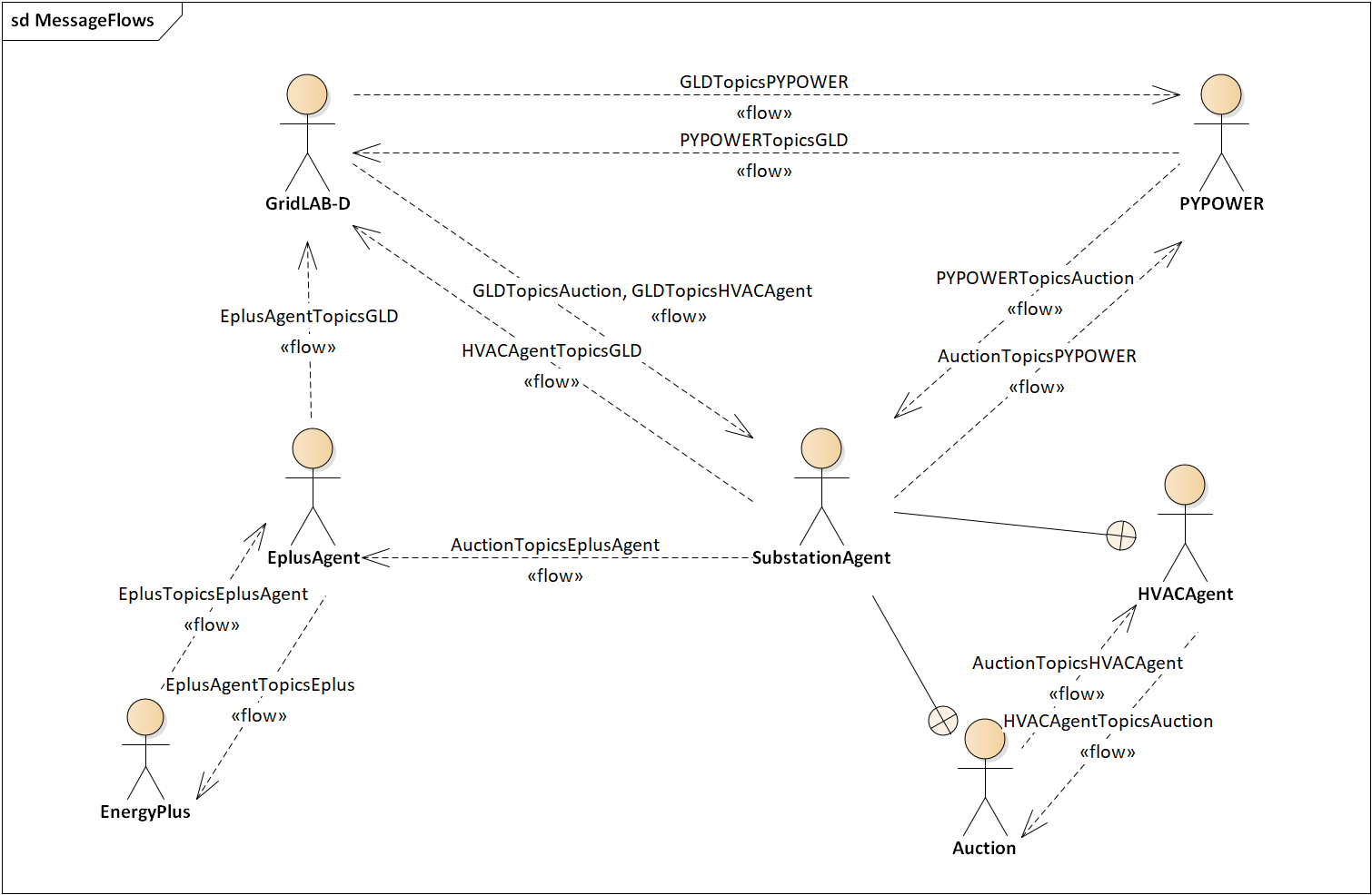
Fig. 61 Message Flows for Simulators and Transactive Agents

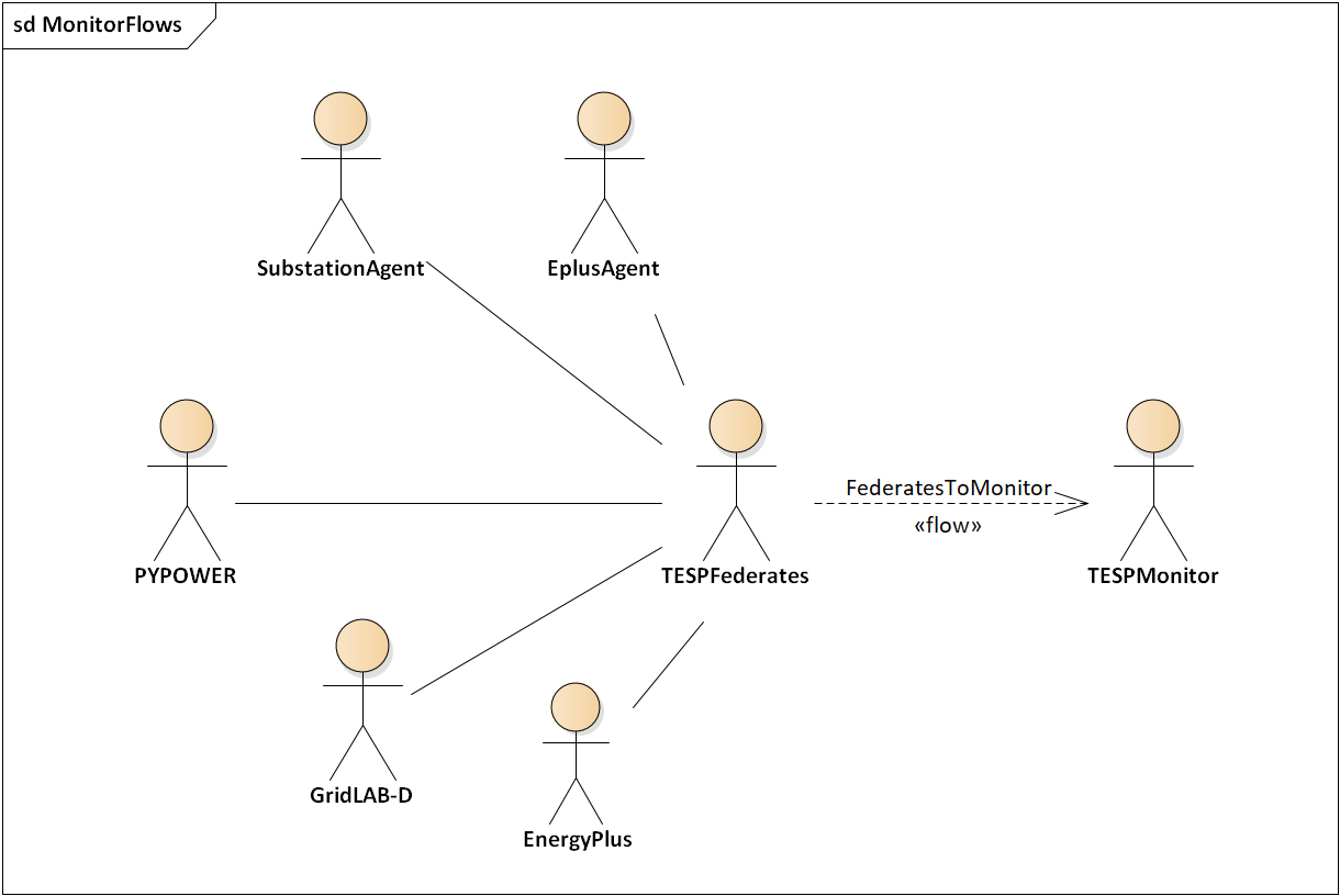
Fig. 62 Message Flows for Solution Monitoring

EnergyPlus publishes three phase power values after each of its solutions (currently on five-minute intervals). These are all numerically equal, at one third of the total building power that includes lights, office equipment, refrigeration and HVAC loads. GridLAB-D subscribes in order to update its power flow model at the point of interconnection for the building, which is typically at a 480-V or 208-V three-phase transformer. EnergyPlus also subscribes to the double-auction market’s published clearing price, using that value for a real-time price (RTP) response of its HVAC load.

Message flows involving the thermostat controller, at the center of Fig. 61, are a little more involved. From the associated house within GridLAB-D, it subscribes to the air temperature, HVAC power state, and the HVAC power if turned on. The controller uses this information to help formulate a bid for electric power at the next market clearing, primarily the price and quantity. Note that each market clearing interval will have its own market id, and that re-bidding may be allowed until that particular market id closes. When bidding closes for a market interval, the double-auction market will settle all bids and publish several values, primarily the clearing price. The house thermostat controllers use that clearing price subscription, compared to their bid price, to adjust the HVAC thermostat setpoint. As noted above, the EnergyPlus building also uses the clearing price to determine how much to adjust its thermostat setting. Fig. 61 shows several other keyword values published by the double-auction market and thermostat controllers; these are mainly used to define “ramps” for the controller bidding strategies. See the GridLAB-D documentation, or TESP design documentation, for more details.

These message schemas are limited to the minimum necessary to operate Version 1, and it’s expected that the schema will expand as new TEAgents are added. Beyond that, note that any of the simulators may subscribe to any values that it “knows about”, i.e., there are no security and access control emulations. This may be a layer outside the scope of TESP. However, there is also no provision for enforcement of bid compliance, i.e. perfect compliance is built into the code. That’s clearly not a realistic assumption, and is within the scope for future versions as described in Section 3.

TESP for Agent Developers

The left-hand portion of Fig. 63 shows the main simulators running in TESP and communicating over HELICS. For the DSO+T study, PYPOWER will be upgraded to AMES and EnergyPlus will be upgraded to a Modelica-based large-building simulator. The large-building agent will also be updated. The current large-building agent is written in C++. It’s functionality is to write metrics from EnergyPlus, and also to adjust a thermostat slider for the building. However, it does not formulate bids for the building. The right-hand portion of Fig. 63 shows the other transactive agents implemented in Python. These communicate directly via Python function calls, i.e., not over HELICS. There are several new agents to implement for the DSO+T study, and this process will require four main tasks:

1 - Define the message schema for information exchange with GridLAB-D, AMES or other HELICS federates. The SubstationAgent will actually manage the HELICS messages, i.e., the agent developer will not be writing HELICS interface code.

2 - Design the agent initialization from metadata available in the GridLAB-D or other dictionaries, i.e., from the dictionary JSON files.

3 - Design the metadata for any intermediate metrics that the agent should write (to JSON files) at each time step.

4 - Design and implement the agent code as a Python class within tesp_support. The SubstationAgent will instantiate this agent class at runtime, and call the class as needed in a time step.

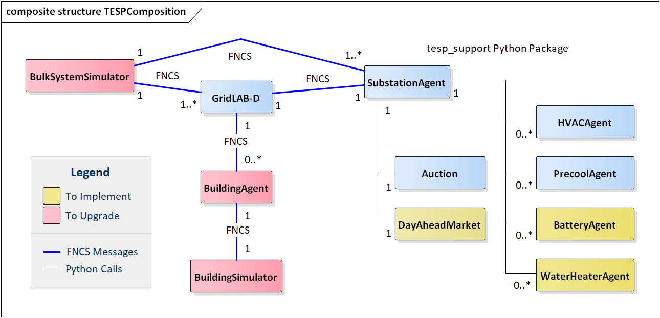
Fig. 63 Composition of Federates in a Running TESP Simulation

Fig. 64 the sequence of interactions between GridLAB-D, the SubstationAgent (encapsulating HVAC controllers and a double-auction market) and PYPOWER. The message hops over HELICS each consume one time step. The essential messages for market clearing are highlighted in red. Therefore, it takes 3 HELICS time steps to complete a market clearing, from the collection of house air temperatures to the adjustment of thermostat setpoints. Without the encapsulating SubstationAgent, two additional HELICS messages would be needed. The first would occur between the self-messages AgentBids and Aggregate, routed between separate HVACController and Auction swimlanes. The second would occur between ClearMarket and AdjustSetpoints messages, also routed between separate Auction and HVACController swimlanes. This architecture would produce additional HELICS message traffic, and also increase the market clearing latency from 3 HELICS time steps to 5 HELICS time steps.

Before and after each market clearing, GridLAB-D and PYPOWER will typically exchange substation load and bus voltage values several times, for each power flow (PF) solution. These HELICS messages are indicated in black; they represent much less traffic than the market clearing messages.

Some typical default time steps are:

1 - 5 seconds, for HELICS, leading to a market clearing latency of 15 seconds

2 - 15 seconds, for GridLAB-D and PYPOWER’s regular power flow (PF)

3 - 300 seconds, for spot-market clearing, PYPOWER’s optimal power flow (OPF), EnergyPlus (not shown in Fig. 64) and the metrics aggregation.

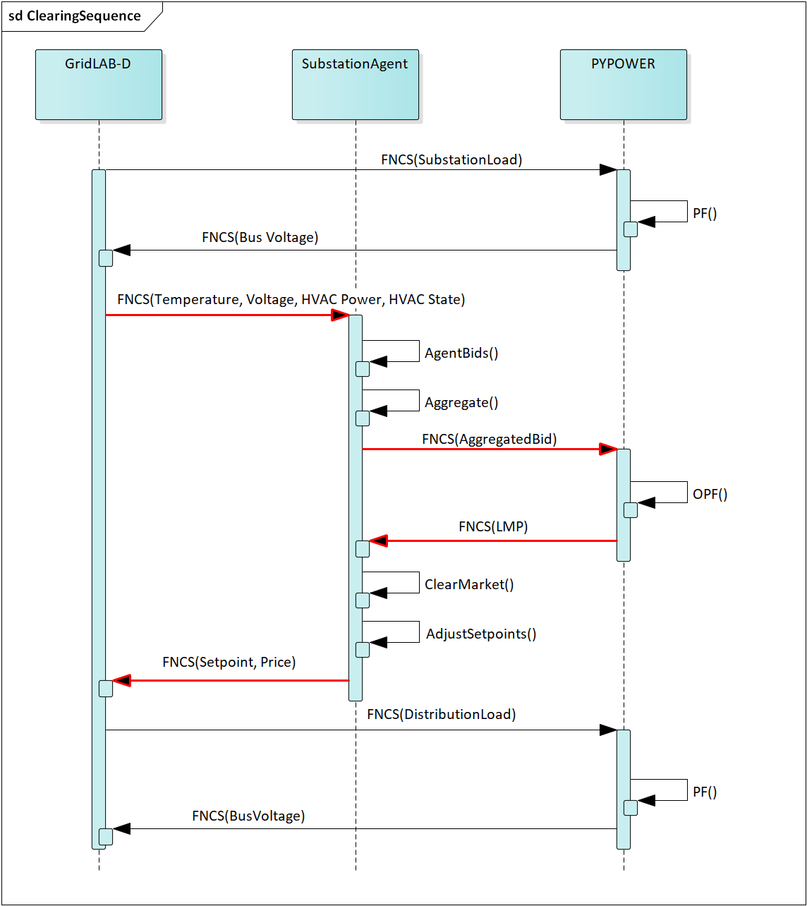
Fig. 64 HELICS Message Hops around Market Clearing Time

Output Metrics to Support Evaluation

TESP will produce various outputs that support comparative evaluation of different scenarios. Many of these outputs are non-monetary, so a user will have to apply different weighting and aggregation methods to complete the evaluations. This is done in the Evaluation Script, which is written in Python. These TESP outputs all come from the Operational Model, or from the Growth Model applied to the Operational Model. For efficiency, each simulator writes intermediate metrics to Javascript Object Notation (JSON) files during the simulation, as shown in Figure 5. For example, if GridLAB-D simulates a three-phase commercial load at 10-second time steps, the voltage metrics output would only include the minimum, maximum, mean and median voltage over all three phases, and over a metrics aggregation interval of 5 to 60 minutes. This saves considerable disk space and processing time over the handling of multiple CSV files. Python, and other languages, have library functions optimized to quickly load JSON files.

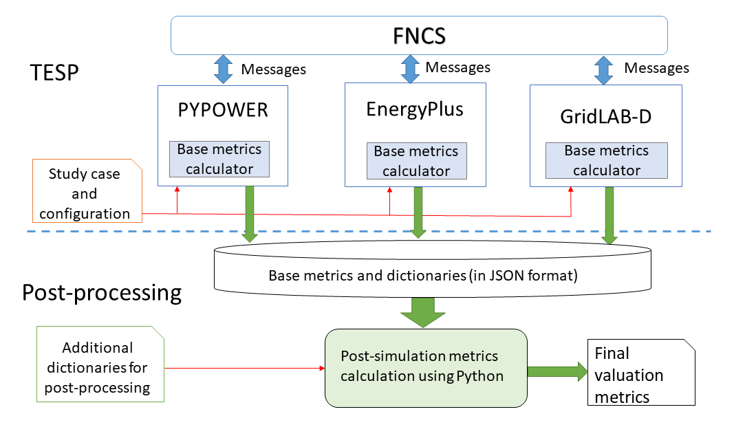
Fig. 65 Partitioning the valuation metrics between simulation and post-processing

To support these intermediate metrics, two new classes were added to the “tape” module of GridLAB-D, as shown in Fig. 66. The volume and variety of metrics generated from GridLAB-D is currently the highest among simulators within TESP, so it was especially important here to provide outputs that take less time and space than CSV files. Most of the outputs come from billing meters, either single-phase triplex meters that serve houses, or three-phase meters that serve commercial loads. The power, voltage and billing revenue outputs are linked to these meters, of which there may be several thousand on a feeder. Houses, which always connect to triplex meters, provide the air temperature and setpoint deviation outputs for evaluating occupant comfort. Inverters, which always connect to meters, provide real and reactive power flow outputs for connected solar panels, battery storage, and future DER like vehicle chargers. Note that inverters may be separately metered from a house or commercial building, or combined on the same meter as in net metering. Feeder-level metrics, primarily the real and reactive losses, are also collected by a fourth class that iterates over all transformers and lines in the model; this substation-level class has just one instance not shown in Fig. 66. An hourly metrics output interval is shown, but this is adjustable.

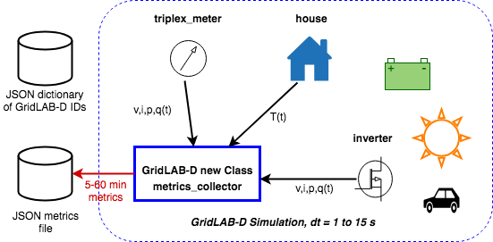
Fig. 66 New metrics collection classes for GridLAB-D

The initial GridLAB-D metrics are detailed in five UML diagrams, so we begin the UML metric descriptions with PYPOWER, which is much simpler. During each simulation, PYPOWER will produce two JSON files, one for all of the generators and another for all of the HELICS interface buses to GridLAB-D. A third JSON file, called the dictionary, is produced before the simulation starts from the PYPOWER case input file. The dictionary serves as an aid to post-processing. Fig. 67 shows the schema for all three PYPOWER metrics files.

The PYPOWER dictionary (top of Fig. 67) includes the system MVA base (typically 100) and GridLAB-D feeder amplification factor. The amplification factor is used to scale up the load from one simulated GridLAB-D feeder to represent many similar feeders connected to the same PYPOWER bus. Each generator has a bus number (more than one generator can be at a bus), power rating, cost function f(P) = c ₀ + c ₁ P + c ₂ P ², startup cost, shutdown cost, and other descriptive information. Each DSOBus has nominal P and Q that PYPOWER can vary outside of GridLAB-D, plus the name of a GridLAB-D substation that provides additional load at the bus. In total, the PYPOWER dictionary contains four JSON objects; the ampFactor, the baseMVA, a dictionary (map) of Generators keyed on the generator id, and a dictionary (map) of DSOBuses keyed on the bus id. In PYPOWER, all id values are integers, but the other simulators use string ids.

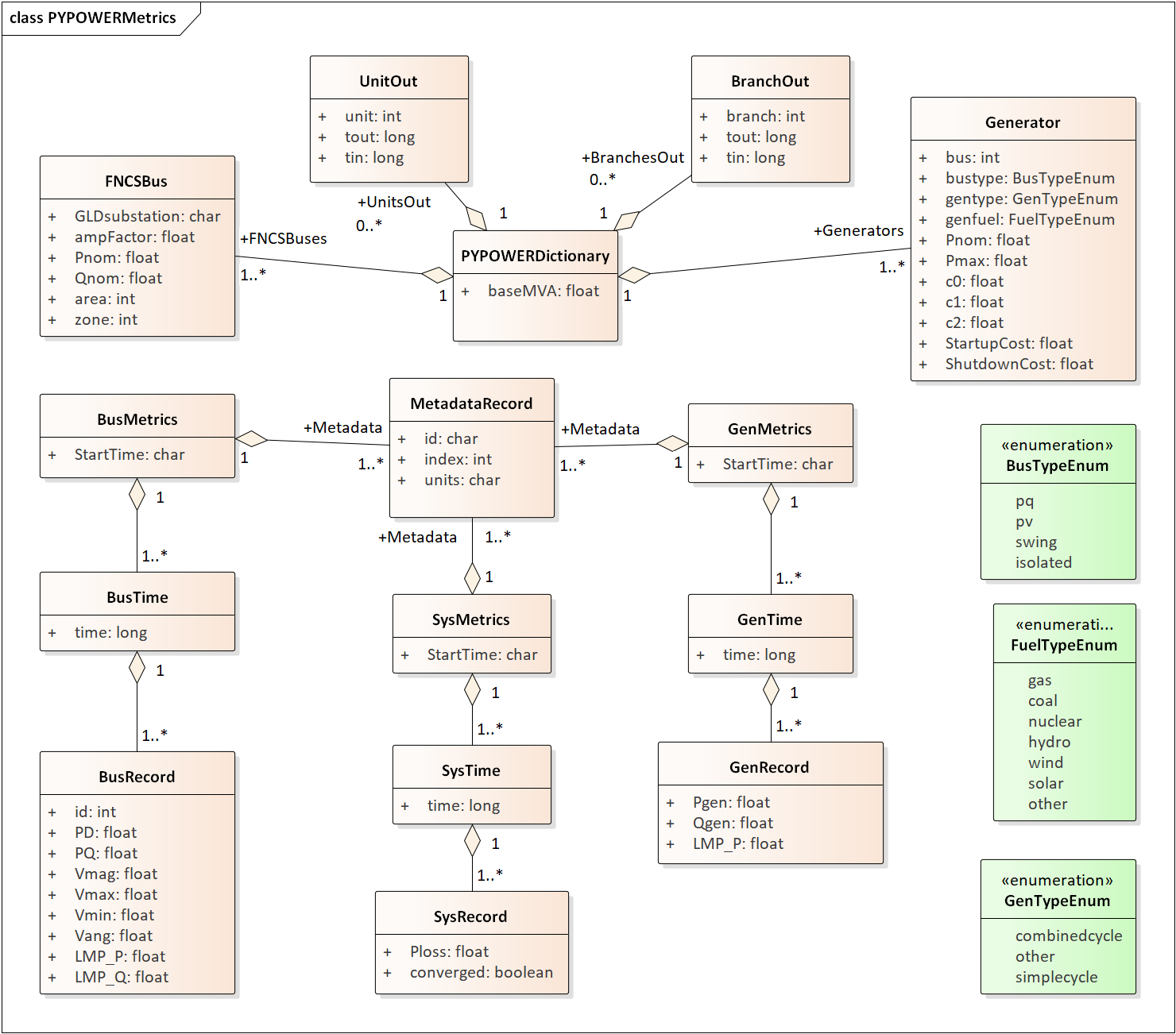
Fig. 67 PYPOWER dictionary with generator and DSO bus metrics

The GenMetrics file (center of Fig. 67) includes the simulation starting date, time and time zone as StartTime, which should be the same in all metrics output files from that simulation. It also contains a dictionary (map) of three MetadataRecords, which define the array index and units for each of the three generator metric output values. These are the real power LMP, along with the actual real and reactive power outputs, Pgen and Qgen. At each time for metrics output, a GenTime dictionary (map) object will be written with key equal to the time in seconds from the simulation StartTime, and the value being a dictionary (map) of GenRecords.

The GenRecord keys are generator numbers, which will match the dictionary. The GenRecord values are arrays of three indexed output values, with indices and units matching the Metadata. This structure minimizes nesting in the JSON file, and facilitates quick loading in a Python post-processor program. Valuation may require the use of both metrics and the dictionary. For example, suppose we need the profit earned by a generator at a time 300 seconds after the simulation starting time. The revenue comes from the metrics as LMP_P * Pgen. In order to find the cost, one would start with cost function coefficients obtained from the dictionary for that generator, and substitute Pgen into that cost function. In addition, the post processing script should add startup and shutdown costs based on Pgen transitions between zero and non-zero values; PYPOWER itself does not handle startup and shutdown costs. Furthermore, aggregating across generators and times would have to be done in post-processing, using built-in functions from Python’s NumPy package. The repository includes an example of how to do this.

Turning to more complicated GridLAB-D metrics, Fig. 68 provides the dictionary. At the top level, it includes the substation transformer size and the PYPOWER substation name for HELICS connection. There are four dictionaries (maps) of component types, namely houses, inverters, billing meters and feeders. While real substations often have more than one feeder, in this model only one feeder dictionary will exist, comprising all GridLAB-D components in that model. The reason is that feeders are actually distinguished by their different circuit breakers or reclosers at the feeder head, and GridLAB-D does not currently associate components to switches that way. In other words, there is one feeder and one substation per GridLAB-D file in this version of TESP. When this restriction is lifted in a future version, attributes like feeder_id, house_count and inverter_count will become helpful. At present, all feeder_id attributes will have the same value, while house_count and inverter_count will simply be the length of their corresponding JSON dictionary objects. Fig. 68 shows that a BillingMeter must have at least one House or Inverter with no upper limit, otherwise it would not appear in the dictionary. The wh_gallons attribute can be used to flag a thermostat-controlled electric waterheater, but these are not yet treated as responsive loads in Version 1. Other attributes like the inverter’s rated_W and the house’s sqft could be useful in weighting some of the metric outputs.

Fig. 69 shows the structure of substation metrics output from GridLAB-D, consisting of real power and energy, reactive power and energy, and losses from all distribution components in that model. As with PYPOWER metrics files, the substation metrics JSON file contains the StartTime of the simulation, Metadata with array index and units for each metric value, and a dictionary (map) of time records, keyed on the simulation time in seconds from StartTime. Each time record contains a dictionary (map) of SubstationRecords, each of which contains an array of 18 values. This structure, with minimal nesting of JSON objects, was designed to facilitate fast loading and navigation of arrays in Python. The TESP code repository includes examples of working with metrics output in Python. Fig. 70 and Fig. 71 show how capacitor switching and regulator tap changing counts are captured as metrics.

Fig. 72 shows the structure of billing meter metrics, which is very similar to that of substation metrics, except that each array contains 30 values. The billing meter metrics aggregate real and reactive power for any houses and inverters connected to the meter, with several voltage magnitude and unbalance metrics. The interval bill is also included, based on metered consumption and the tariff that was input to GridLAB-D. In some cases, revenues may be recalculated in post-processing to explore different tariff designs. It’s also possible to re-calculate the billing determinants from metrics that have been defined.

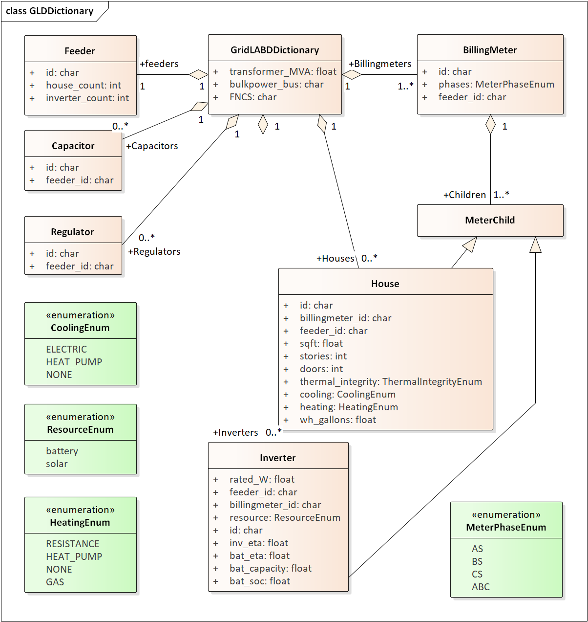
Fig. 68 GridLAB-D dictionary

The Range A and Range B metrics in Fig. 72 refer to ANSI C84.1 [3]. For service voltages less than 600 V, Range A is +/- 5% of nominal voltage for normal operation. Range B is -8.33% to +5.83% of nominal voltage for limited-extent operation. Voltage unbalance is defined as the maximum deviation from average voltage, divided by average voltage, among all phases present. For three-phase meters, the unbalance is based on line-to-line voltages, because that is how motor voltage unbalance is evaluated. For triplex meters, unbalance is based on line-to-neutral voltages, because there is only one line-to-line voltage. In Fig. 72, voltage_ refers to the line-to-neutral voltage, while voltage12_ refers to the line-to-line voltage. The below_10_percent voltage duration and count metrics indicate when the billing meter has no voltage. That information would be used to calculate reliability indices in post-processing, with flexible weighting and aggregation options by customer, owner, circuit, etc. These include the System Average Interruption Frequency Index (SAIFI) and System Average Interruption Duration Index (SAIDI) [17, 18]. This voltage-based approach to reliability indices works whether the outage resulted from a distribution, transmission, or bulk generation event. The voltage-based metrics also support Momentary Average Interruption Frequency Index (MAIFI) for shorter duration outages.

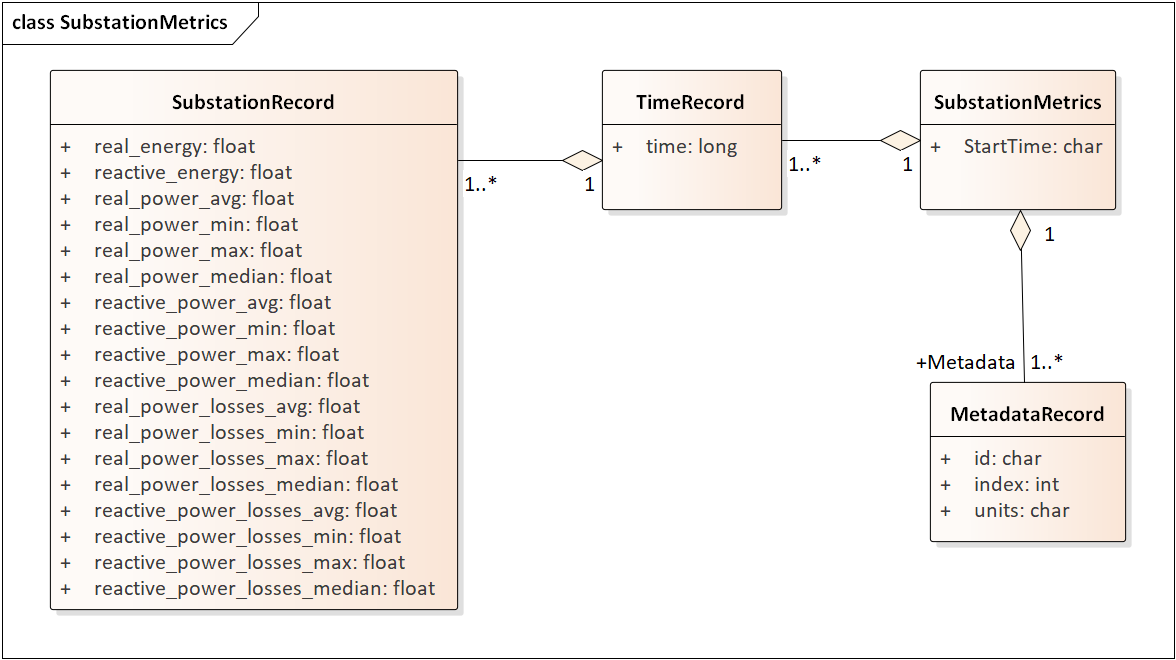
Fig. 69 GridLAB-D substation metrics

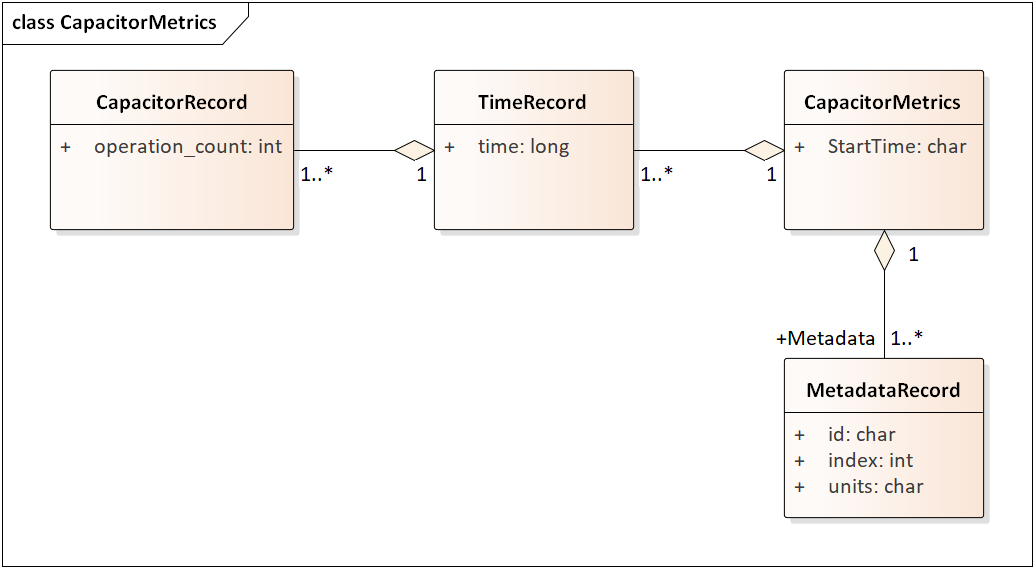
Fig. 70 GridLAB-D capacitor switching metrics

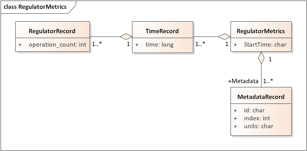
Fig. 71 GridLAB-D regulator tap changing metrics

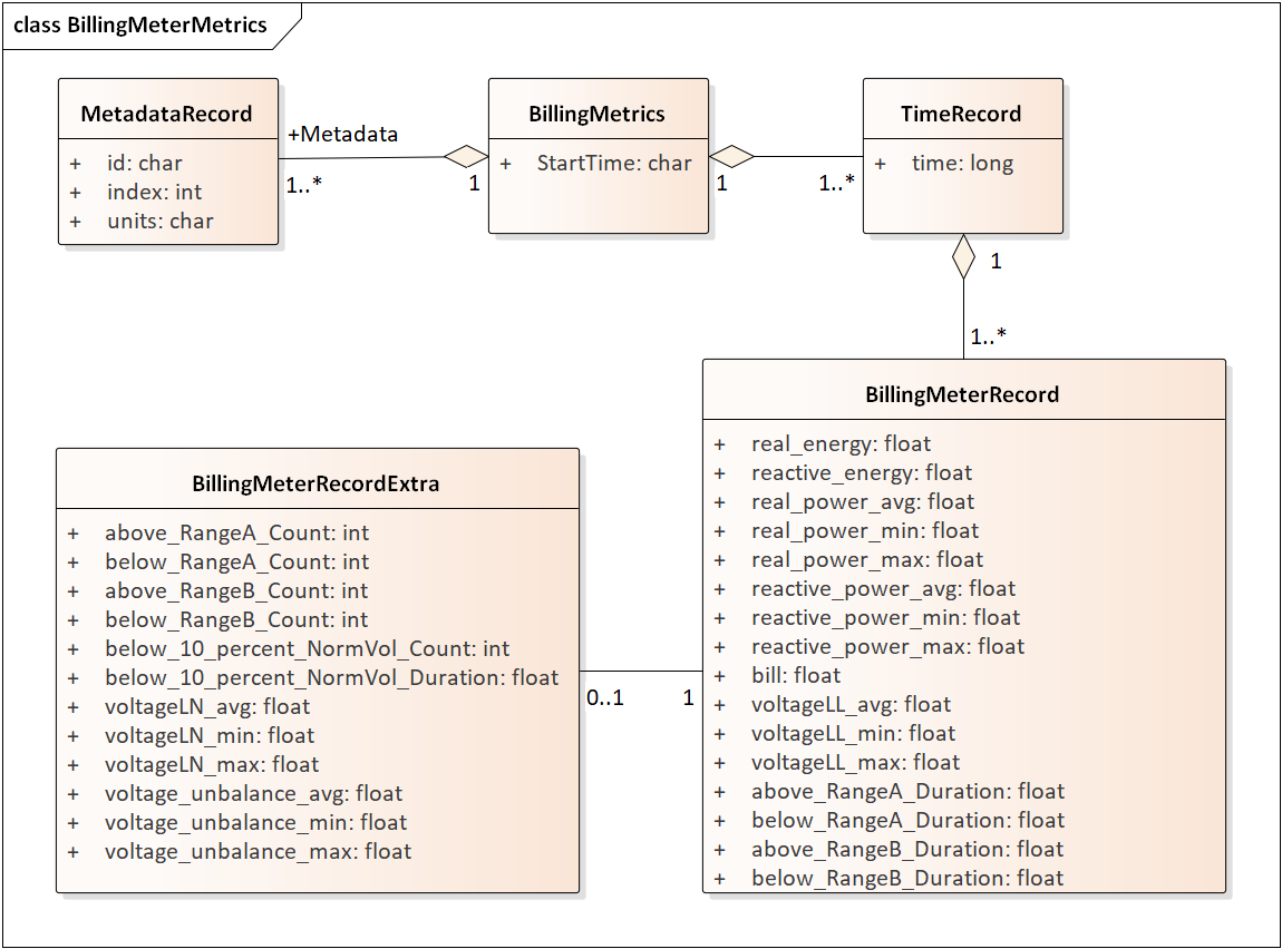
Fig. 72 GridLAB-D billing meter metrics

The house metric JSON file structure is shown in Fig. 73, following the same structure as the other GridLAB-D metrics files, with 18 values in each array. These relate to the breakdown of total house load into HVAC and waterheater components, which are both thermostat controlled. The house air temperature, and its deviation from the thermostat setpoint, are also included. Note that the house bill would be included in billing meter metrics, not the house metrics. Inverter metrics in Fig. 74 include 8 real and reactive power values in the array, so the connected resource outputs can be disaggregated from the billing meter outputs, which always net the connected houses and inverters. In Version 1, the inverters will be net metered, or have their own meter, but they don’t have transactive agents yet.

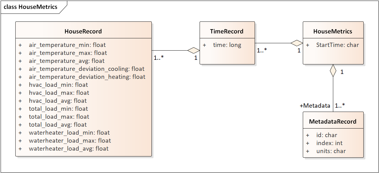
Fig. 73 GridLAB-D house metrics

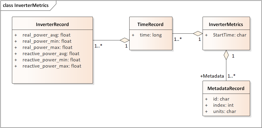
Fig. 74 GridLAB-D inverter metrics

Sample of resulting JSON:

{
"Metadata": {
    "reactive_power_avg": {
        "index": 5,
        "units": "VAR"
    },
    "reactive_power_max": {
        "index": 4,
        "units": "VAR"
    },
    "reactive_power_min": {
        "index": 3,
        "units": "VAR"
    },
    "real_power_avg": {
        "index": 2,
        "units": "W"
    },
    "real_power_max": {
        "index": 1,
        "units": "W"
    },
    "real_power_min": {
        "index": 0,
        "units": "W"
    }
},
"StartTime": "2013-07-01 00:00:00 PDT",
"10200": {
    "battery_inverter_house10_R1_12_47_1_tm_157": [
        -0.0,
        -0.0,
        0.0,
        0.0,
        0.0,
        0.0
    ],
    "battery_inverter_house10_R1_12_47_1_tm_273": [
        -0.0,
        -0.0,
        0.0,
        0.0,
        0.0,
        0.0
    ],
    ...
    }
"10500": {
    "battery_inverter_house10_R1_12_47_1_tm_157": [
        -0.0,
        -0.0,
        0.0,
        0.0,
        0.0,
        0.0
    ],
    ...
    }
}

Fig. 75 shows the transactive agent dictionary and metrics file structures. Currently, these include one double-auction market per substation and one double-ramp controller per HVAC. Each dictionary (map) is keyed to the controller or market id. The Controller dictionary (top left) has a houseName for linkage to a specific house within the GridLAB-D model. In Version 1, there can be only one Market instance per GridLAB-D model, but this will expand in future versions. See the GridLAB-D market module documentation for information about the other dictionary attributes.

There will be two JSON metrics output files for TEAgents during a simulation, one for markets and one for controllers, which are structured as shown at the bottom of Fig. 75. The use of StartTime and Metadata is the same as for PYPOWER and GridLAB-D metrics. For controllers, the bid price and quantity (kw, not kwh) is recorded for each market clearing interval’s id. For auctions, the actual clearing price and type are recorded for each market clearing interval’s id. That clearing price applies throughout the feeder, so it can be used for supplemental revenue calculations until more agents are developed.

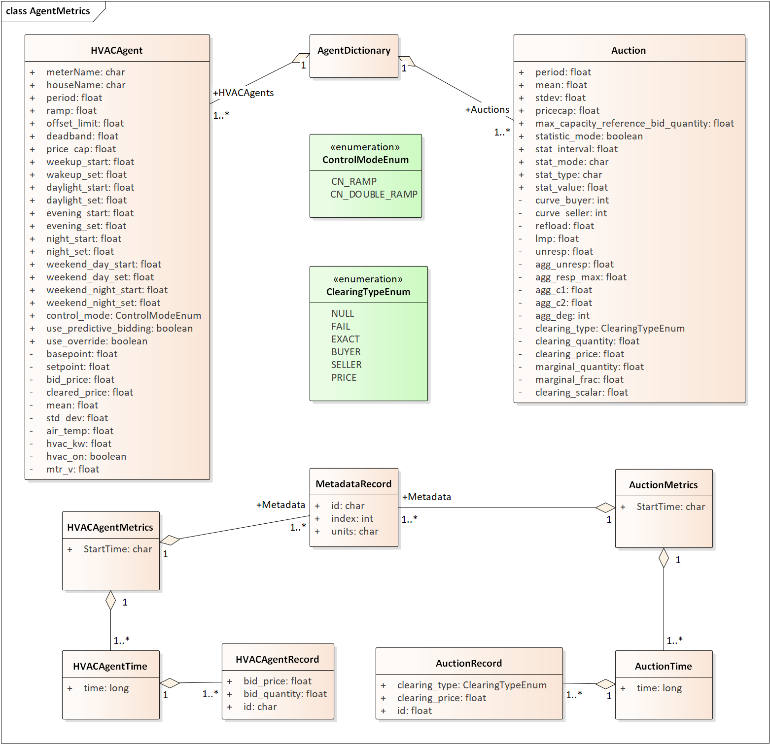
Fig. 75 TEAgent dictionary and metrics

The EnergyPlus dictionary and metrics structure in Fig. 76 follows the same pattern as PYPOWER, GridLAB-D and TEAgent metrics. There are 42 metric values in the array, most of them pertaining to heating and cooling system temperatures and states. Each EnergyPlus model is custom-built for a specific commercial building, with detailed models of the HVAC equipment and zones, along with a customized Energy Management System (EMS) program to manage the HVAC. Many of the metrics are specified to track the EMS program performance during simulation. In addition, the occupants metric can be used for weighting the comfort measures; EnergyPlus estimates the number of occupants per zone based on hour of day and type of day, then TESP aggregates for the whole building. The electric_demand_power metric is the total three-phase power published to GridLAB-D, including HVAC and variable loads from lights, refrigeration, office equipment, etc. The kwhr_price will correspond to the market clearing price from Fig. 75. Finally, the ashrae_uncomfortable_hours is based on a simple standardized model, aggregated for all zones [4].

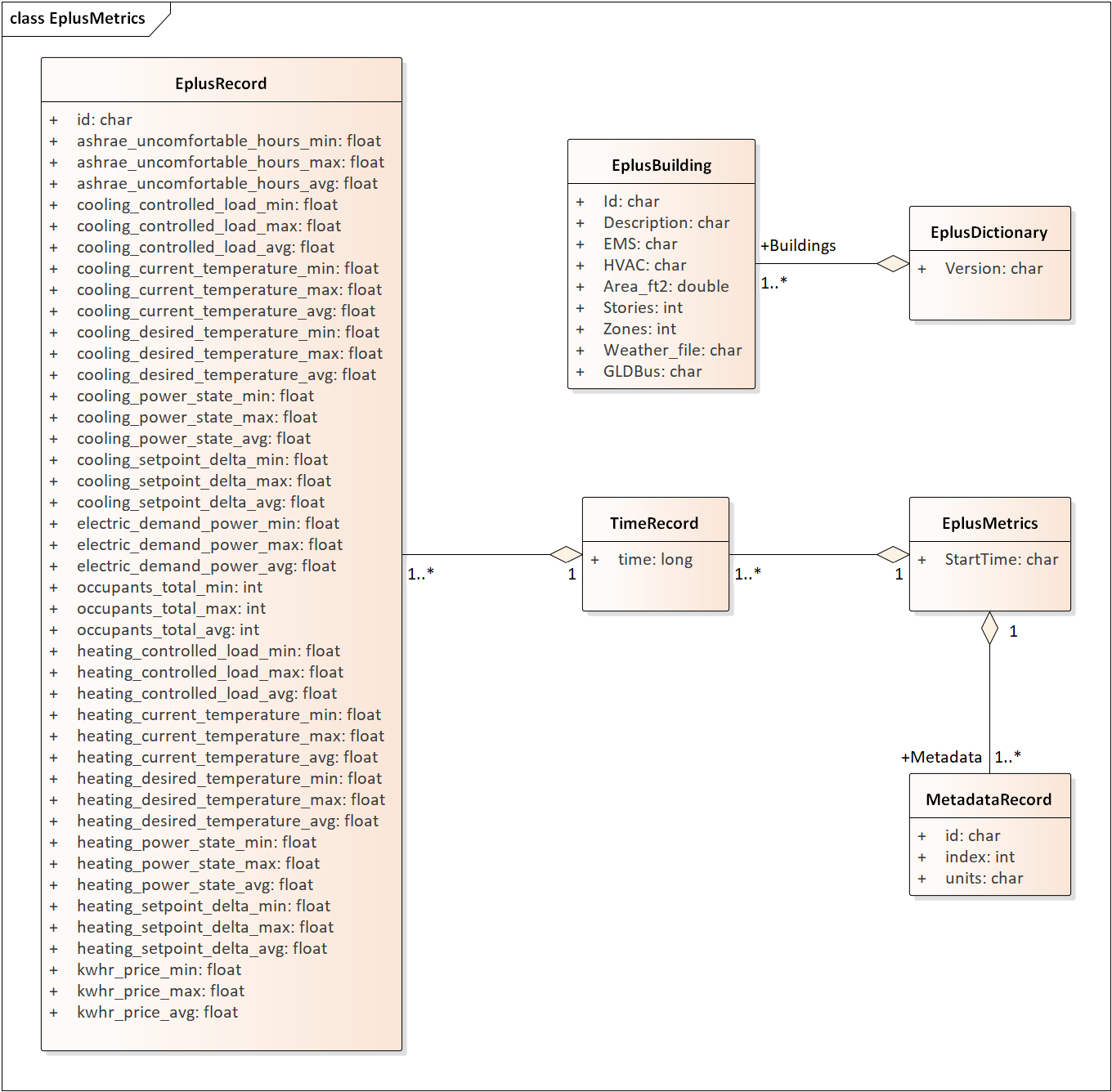
Fig. 76 EnergyPlus dictionary and metrics

GridLAB-D Enhancements

The TSP simulation task includes maintenance and updates to GridLAB-D in support of TESP. This past year, the GridLAB-D enhancements done for TESP have included:

1. Extraction of the double-auction market and double-ramp controller into separate modules, with communication links to the internal GridLAB-D houses. This pattern can be reused to open up other GridLAB-D controller designs to a broader community of developers.

2. Porting the FNCS-enabled version of GridLAB-D to Microsoft Windows. This had not been working with the MinGW compiler that was recently adopted for GridLAB-D on Windows, and it will be important for other projects.

3. Implementing the JSON metrics collector and writer classes in the tape module. This should provide efficiency and space benefits to other users who need to post-process GridLAB-D outputs.

4. Implementing a JSON-based message format for agents running under FNCS. Again, this should provide efficiency benefits for other projects that need more complicated FNCS message structures.

Developing Valuation Scripts

In order to provide new or customized valuation scripts in Python, the user should first study the provided examples. These illustrate how to load the JSON dictionaries and metrics described in Section 1.5, aggregate and post-process the values, make plots, etc. Coupled with some experience or learning in Python, this constitutes the easiest route to customizing TESP.

Developing Agents

The existing auction and controller agents provide examples on how to configure the message subscriptions, publish values, and link with HELICS at runtime. Section 1.4 describes the existing messages, but these constitute a minimal set for Version 1. It’s possible to define your own messages between your own TEAgents, with significant freedom. It’s also possible to publish and subscribe, or “peek and poke”, any named object / attribute in the GridLAB-D model, even those not called out in Section 1.4. For example, if writing a waterheater controller, you should be able to read its outlet temperature and write its tank setpoint via HELICS messages, without modifying GridLAB-D code. You probably also want to define metrics for your TEAgent, as in Section 1.5. Your TEAgent will run under supervision of a HELICS broker program. This means you can request time steps, but not dictate them. The overall pattern of a HELICS-compliant program will be:

1. Initialize HELICS and subscribe to messages, i.e. notify the broker.

2. Determine the desired simulation stop_time, and any time step size (delta_t) preferences. For example, a transactive market mechanism on 5-minute clearing intervals would like delta_t of 300 seconds.

3. Set time_granted to zero; this will be under control of the HELICS broker.

4. Initialize time_request; this is usually 0 + delta_t, but it could be stop_time if you just wish to collect messages as they come in.

5. While time_granted < stop_time:

   1. Request the next time_request from HELICS; your program then blocks.

   2. HELICS returns time_granted, which may be less than your time_request. For example, controllers might submit bids up to a second before the market interval closes, and you should keep track of these.

   3. Collect and process the messages you subscribed to. There may not be any if your time request has simply come up. On the other hand, you might receive bids or other information to store before taking action on them.

   4. Perform any supplemental processing, including publication of values through HELICS. For example, suppose 300 seconds have elapsed since the last market clearing. Your agent should settle all the bids, publish the clearing price (and other values), and set up for the next market interval.

   5. Determine the next time_request, usually by adding delta_t to the last one. However, if time_granted has been coming irregularly in 5b, you might need to adjust delta_t so that you do land on the next market clearing interval. If your agent is modeling some type of dynamic process, you may also adapt delta_t to the observed rates of change.

   6. Loop back to 5a, unless time_granted >= stop_time.

6. Write your JSON metrics file; Python has built-in support for this.

7. Finalize HELICS for an orderly shutdown, i.e. notify the broker that you’re done.

The main points are to realize that an overall “while loop” must be used instead of a “for loop”, and that the time_granted values don’t necessarily match the time_requested values.

Developers working with C/C++ will need much more familiarity with compiling and linking to other libraries and applications, and much more knowledge of any co-simulators they wish to replace. This development process generally takes longer, which represents added cost. The benefits could be faster execution times, more flexibility in customization, code re-use, etc.

tesp_support Package Design

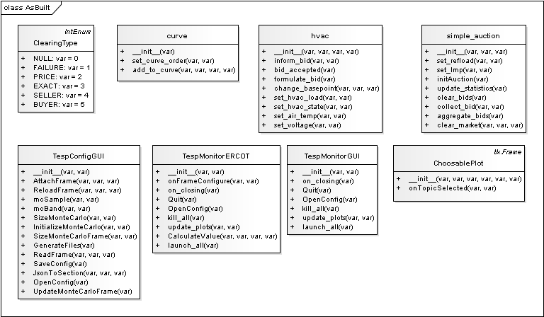
Fig. 77 Classes in the tesp_support package.

Development Work Flow for tesp_support

This is the main code repository for Python-based components of TESP, including the transactive agents, case configuration and post-processing. Currently, there are three kinds of transactive agent implemented here:

1. double-auction spot market, typically runs every 5 to 15 minutes

2. an electric cooling controller based on the Olympic Peninsula double-ramp method

3. an electric pre-cooling controller used to mitigate overvoltages in the NIST TE Challenge Phase 2

To develop a new agent, you may choose to copy an example Python file from this directory into your own test directory, to serve as a starting point. When finished, you should integrate the agent into this tesp_support package, so it will be available to other TESP developers and users. In this re-integration process, you also need to modify api.py so that other Python code can call your new agent, and test it that way before re-deploying tesp_support to PyPi. Also review setup.py in the parent directory to make sure you’ve included any new dependencies, including version updates.

A second method is to create your new file(s) in this directory, which integrates your new agent from the start. There will be some startup effort in modifying api.py and writing the script/batch files to call your agent from within your working test directory. It may pay off in the end, by reducing the effort and uncertainty of code integration at the end.

Suggested sequence of test cases for development:

1. 30-house example at https://github.com/pnnl/tesp/tree/master/examples/te30. This includes one large building, one connection to a 9-bus/4-generator bulk system, and a stiff feeder source. The model size is suited to manual adjustments, and testing the interactions of agents at the level of a feeder or lateral. There are effectively no voltage dependencies or overloads, except possibly in the substation transformer. This case runs on a personal computer in a matter of minutes.

2. 8-bus ERCOT example at https://github.com/pnnl/tesp/tree/master/ercot/case8. This includes 8 EHV buses and 8 distribution feeders, approximately 14 bulk system units, and several thousand houses. Use this for testing your agent configuration from the GridLAB-D metadata, for large-scale interactions and stability, and for interactions with other types of agent in a less controllable environment. This case runs on a personal computer in a matter of hours.

3. 200-bus ERCOT example, when available. This will have about 600 feeders with several hundred thousand houses, and it will probably have to run on a HPC. Make sure the code works on the 30-house and 8-bus examples first.

• From this directory, ‘pip install -e .’ points Python to this cloned repository for any calls to tesp_support functions

• See the https://github.com/pnnl/tesp/tree/master/src/tesp_support/tesp_support for a roadmap of existing Python source files, and some documentation. Any changes or additions to the code need to be made in this directory.

• Run tests from any other directory on this computer

• When ready, edit the tesp_support version number and dependencies in setup.py

• To deploy, ‘python setup.py sdist upload’

• Any user gets the changes with ‘pip install tesp_support –upgrade’

• Use ‘pip show tesp_support’ to verify the version and location on your computer